Elo & Bradley–Terry: the science behind the World Cup predictor

A refresher on the two rating models this project is built on, how each one is updated, why — at the right parameter values — they are literally the same model, and how that single idea is wired into the World Cup 2026 predictor.

0. The one idea: a pairwise comparison → a strength

Both models answer the same question:

Given that things keep beating each other in pairs, what single number ("strength") should we assign to each one so that the better-rated one is expected to win more often?

Everything else is a parameterization choice (raw vs log strength, base-10 vs base-e) and an estimation choice (update one number after every game → online, or solve for all numbers at once over a batch → offline).

A real match result ("Germany beat Brazil 2–1") and a subjective user pick ("I think Brazil beats Germany") are the same kind of observation: a directed pairwise comparison. So they live in one comparison graph over the same set of teams, with two kinds of edges, and a single strength model is fit on the whole thing.

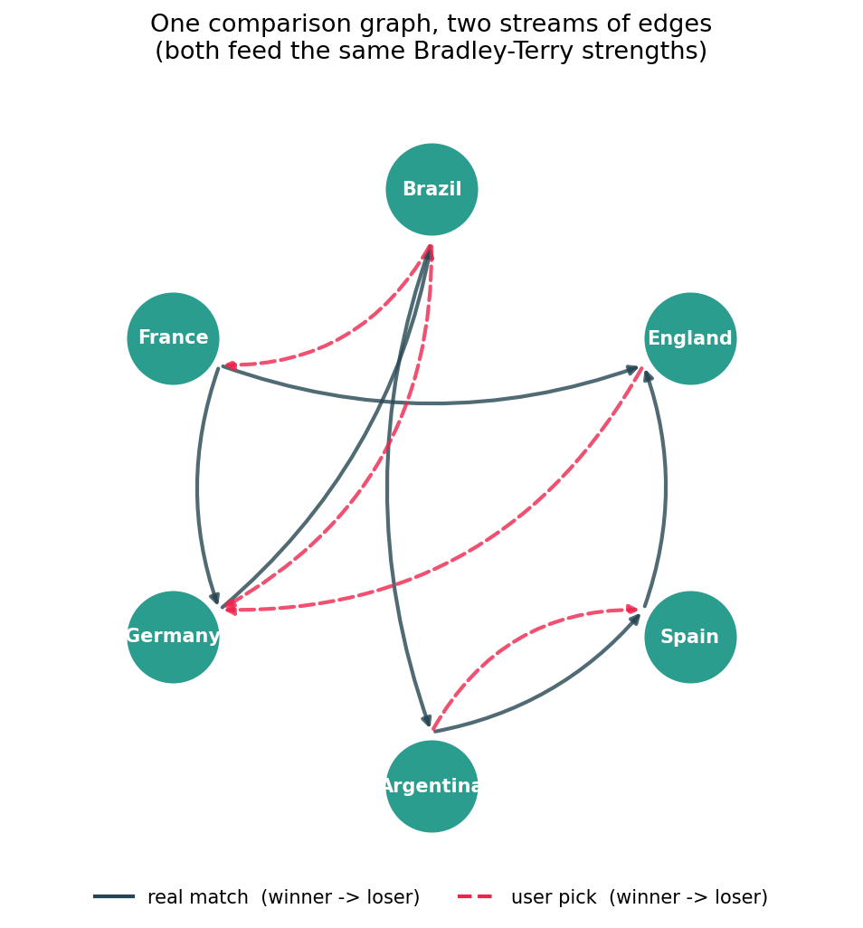
Solid edges are real results, dashed edges are one user's picks. They can disagree (here the user insists Brazil beats Germany even though the data has Germany winning). The fusion step decides who wins that argument, per team, by how much evidence each side brought.

1. Bradley–Terry — the offline / batch model

1.1 The model

Bradley–Terry assigns each item a positive strength p_i. The probability that i beats j is its share of the pair's total strength:

P(i beats j) = p_i / (p_i + p_j)

def bt_prob(p_i, p_j):
    """Probability that i beats j, from raw strengths."""
    return p_i / (p_i + p_j)

That's the whole model. If i is twice as strong as j, it wins 2/3 of the time.

1.2 The log-strength form (this is where Elo lives)

Write each strength as the exponential of a real-valued parameter, p_i = e^(β_i) (so β_i = ln(p_i) is the log-strength). Substitute:

P(i beats j) = e^(β_i) / (e^(β_i) + e^(β_j))
             = 1 / (1 + e^(-(β_i - β_j)))
             = σ(β_i - β_j)

import math

def sigmoid(x):
    return 1 / (1 + math.exp(-x))

def bt_prob_logstrength(beta_i, beta_j):
    """Same model as bt_prob, in log-strength (β) coordinates."""
    return sigmoid(beta_i - beta_j)

So the win probability is a logistic (sigmoid) function of the difference of log-strengths. The raw-strength curve and the log-strength sigmoid are the same model in two coordinate systems:

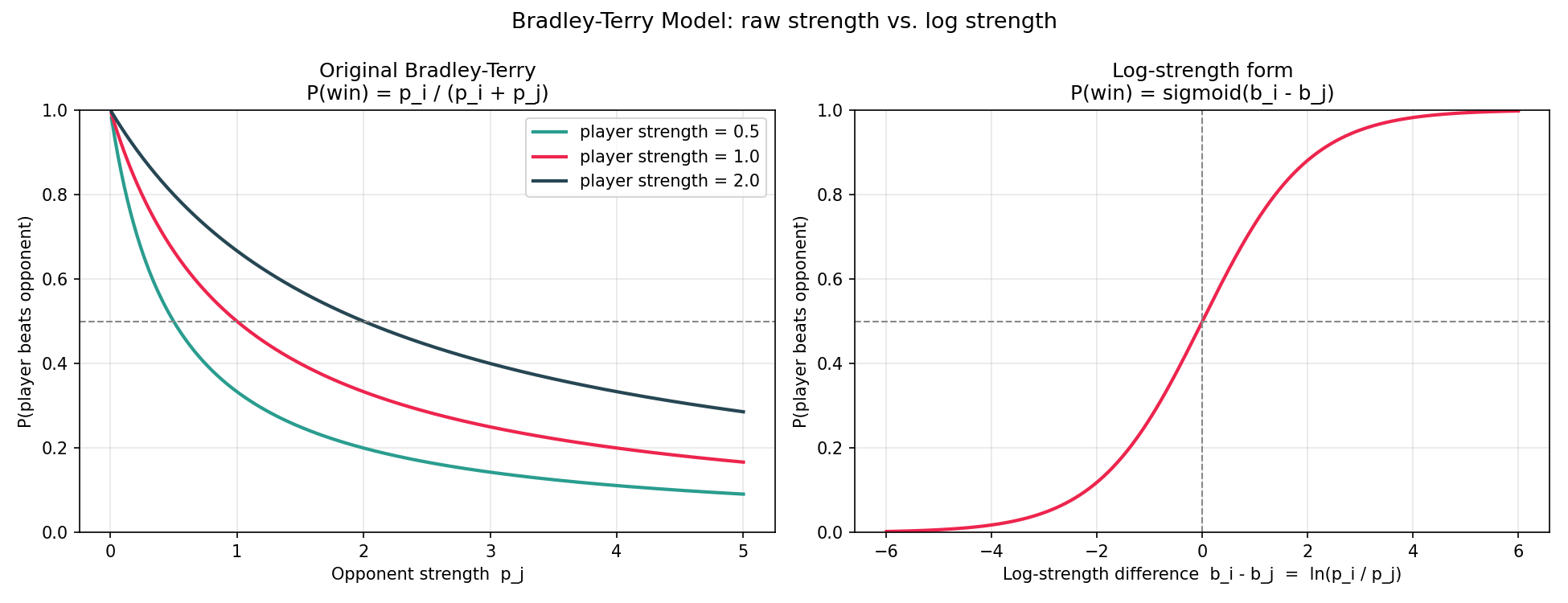
Left: P(win) vs the opponent's raw strength p_j, for a few players. Right: the same thing as a single symmetric sigmoid of the gapβ_i - β_j. That right-hand sigmoid is exactly the shape behind an Elo expected-score curve (see §3).

Only differences of β matter, so the scale has one free constant — we fix it by recentering, e.g. Σ_i β_i = 0 (or geometric-mean strength 1).

1.3 How it is "updated": fit the whole batch at once (MLE)

Bradley–Terry is offline: you take a batch of results and solve for all the strengths θ = (β_1, …, β_n) simultaneously by maximum likelihood. The log-likelihood of a batch of comparisons is

ℓ(θ) = Σ over comparisons [ y · ln σ(β_i - β_j) + (1 - y) · ln(1 - σ(β_i - β_j)) ]

def log_likelihood(theta, comparisons):
    """theta: list of log-strengths. comparisons: list of (i, j, y), y=1 if i won."""
    total = 0.0
    for i, j, y in comparisons:
        p = sigmoid(theta[i] - theta[j])
        total += y * math.log(p) + (1 - y) * math.log(1 - p)
    return total

where y = 1 if i won. The key fact that makes this well-behaved:

ℓ(θ) is concave — it has a single hill, so there is a unique maximum (the MLE), and any hill-climber finds it regardless of where it starts.

θ̂ = argmax_θ ℓ(θ) is the fitted set of strengths. The likelihood is a landscape over all possible strength assignments; the MLE is the location of its summit.

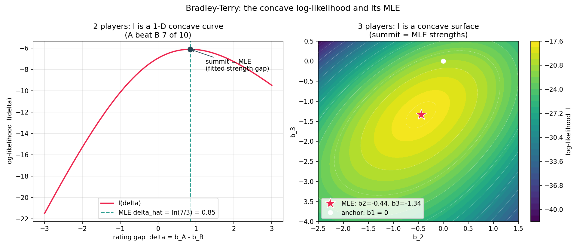
Left: with 2 players, ℓ depends only on the single gap δ = β_A - β_B, a 1-D concave curve whose summit sits at δ̂ = ln(wins / losses) = logit(win rate). Right: with 3 players (one pinned at 0 as the anchor), ℓ is a concave surface; the star marks the MLE strengths.

So the two-player MLE has a clean closed form — if A beat B 7 of 10 times, β_A - β_B = ln(7/3).

1.4 The actual update rule (MM / Zermelo)

For more than two teams there's no closed form, but you don't need a generic optimizer. The classic MM (minorize–maximize), a.k.a. Zermelo iteration is a few lines. Working in raw strengths β_i (the exponentiated log-strengths):

β_i  ←  W_i / Σ_{j≠i} ( n_ij / (β_i + β_j) )

def mm_update(beta, wins, n):
    """One MM/Zermelo sweep. beta: raw strengths, wins[i]: total wins of i,
    n[i][j]: number of times i and j met. Renormalizes to geometric mean 1."""
    size = len(beta)
    new = []
    for i in range(size):
        denom = sum(n[i][j] / (beta[i] + beta[j])
                    for j in range(size) if j != i)
        new.append(wins[i] / denom)
    gmean = math.exp(sum(math.log(b) for b in new) / size)
    return [b / gmean for b in new]

where W_i is i's total wins and n_ij is how many times i and j met. Each sweep updates every team, then renormalizes to geometric mean 1. Because the likelihood is concave this converges to the unique optimum from any start.

Two details matter in practice:

• Regularization adds a virtual half-win against a neutral reference

(strength 1). This shrinks strengths toward the mean so a team that swept its few opponents doesn't fit to an infinite strength — the pure-MLE degeneracy when someone has a 100% record. - Unplayed teams are left at θ = 0 and flagged, so the fusion layer can pin them to the data prior instead of inventing a strength.

2. Elo — the online model

Elo is the same strength idea, but it never stores a batch and never solves a system. It keeps one running number per player and nudges it after every single game. That makes it online.

2.1 Expected score (the same sigmoid, base-10)

Elo predicts the expected score (≈ win probability) of A vs B as

E_A = 1 / (1 + 10^((R_B - R_A) / 400))

def elo_expected(r_a, r_b):
    """Expected score of A against B from Elo ratings."""
    return 1 / (1 + 10 ** ((r_b - r_a) / 400))

This is the Bradley–Terry sigmoid wearing different units: a logistic in the rating gap, with base 10 and a scale of 400 instead of base e and scale 1.

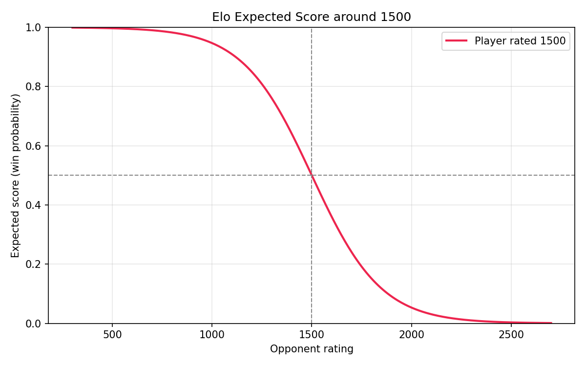
Fix A at 1500, sweep B. Equal ratings → 50%. A 400-point edge → about 91%. The "400" is just the chosen width of the curve.

2.2 The update rule (online gradient step)

After a game, move the rating toward the surprise:

R' = R + K · (S - E)

def elo_update(r, s, e, k=32):
    """New rating after a game. s: actual result (1/0/0.5), e: expected score."""
    return r + k * (s - e)

• S = actual result (1 win, 0 loss, ½ draw),

• E = expected score from the formula above,

• K = K-factor, the maximum swing per game (learning rate).

If you were expected to win (E high) and did, S - E is small → tiny change. Pull off an upset (E low, S = 1) → big jump. The size of the move scales with how surprising the result was.

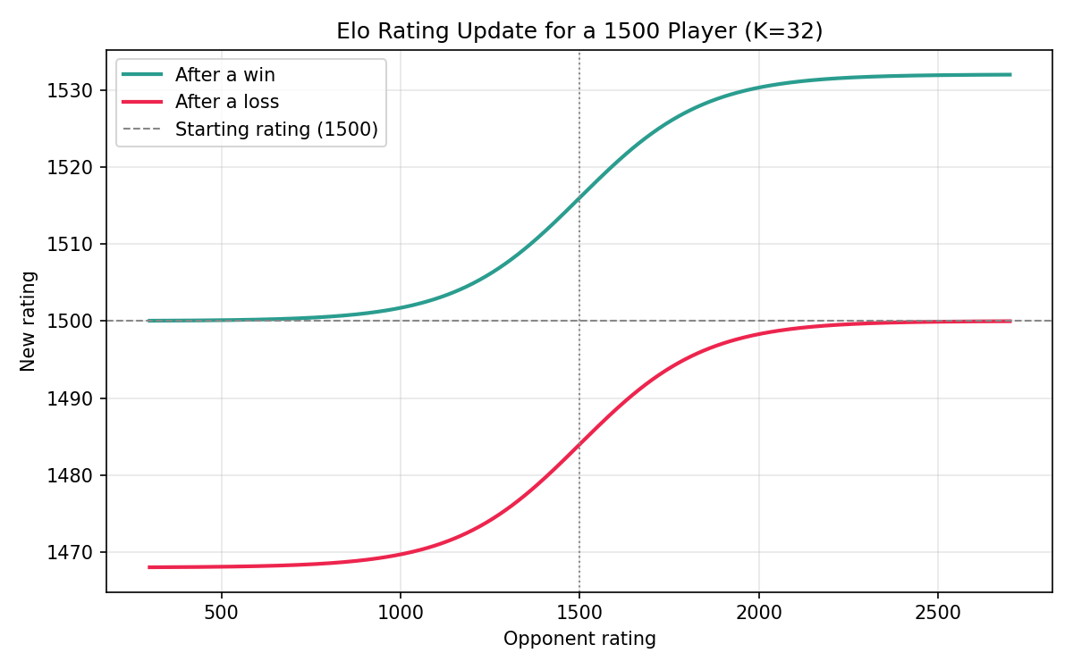
The new rating after a win (green) and a loss (red), sweeping the opponent. Beat a much stronger opponent → the win curve spikes; lose to a much weaker one → the loss curve plunges. The vertical gap between the two curves is exactly K(here 32): the most a single game can ever move you.

This is not a different model from §1 — it is one online stochastic-gradient step on the very same Bradley–Terry log-likelihood, taken one observation at a time. S - E is the gradient of the log-likelihood of that one game with respect to the rating; K is the step size. Elo is "Bradley–Terry by SGD, never batched."

3. Why they are the same model

Bradley–Terry on the Elo rating scale is the Elo curve. Map a rating R onto a strength one of two equivalent ways:

| parameterization | strength | recovers Elo when | |---|---|---| | base-10 | p = 10^(R/400) | always | | natural-log | p = e^(R/S) | S = 400/ln(10) ≈ 173.72 |

Plug either into p_i / (p_i + p_j) and it collapses to the Elo expected score exactly — the only difference is floating-point noise (~10^-16):

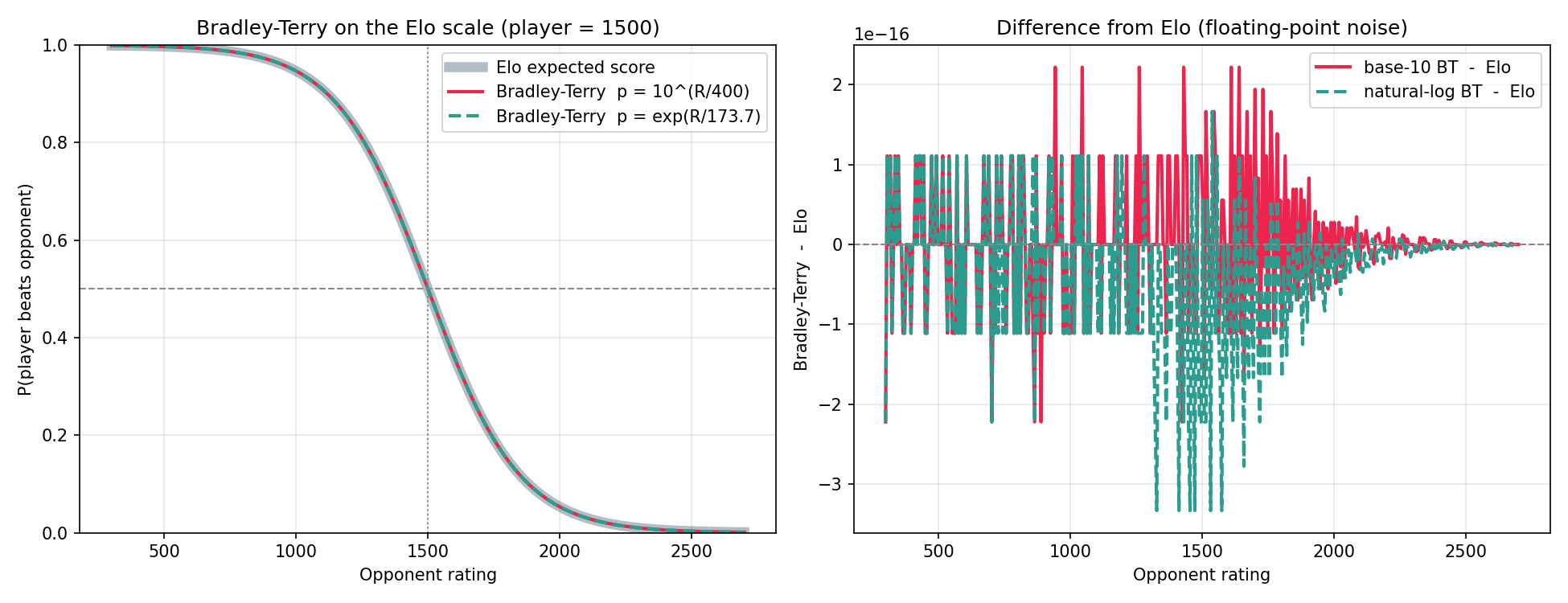
Left: the Elo curve and both BT parameterizations plotted on top of each other; they coincide. Right: residuals vs Elo, which are pure rounding error. The constant S = 400/ln(10) ≈ 173.72 is the exchange rate between "Elo points" and "natural log-strength (θ) units."

So the difference between the two is not the model, it's the estimator:

| | Bradley–Terry | Elo | |---|---|---| | view of the data | a batch of comparisons | a stream, one game at a time | | what's stored | the whole result set, refit on demand | one running number per player | | update | full MLE over the batch (MM/Zermelo, §1.4) | one SGD step R' = R + K(S - E) (§2.2) | | parameter | log-strength β (natural log) | rating R (base-10, ×173.7 = β) | | optimum | unique (concave likelihood) | tracks the same optimum, noisily, online |

The reason this matters in practice: a sequence of Elo updates with a decaying K converges to the batch Bradley–Terry MLE. Elo is the online shadow of the offline fit. The predictor exploits this freely — it fits the data prior offline with batch BT, and updates the user's beliefs online with Elo-style steps, knowing the two live on one shared θ scale.

4. How the World Cup predictor uses all this

The 2026 format is 48 teams in 12 groups of 4, group stage → knockout, with group ties broken on goal difference, then goals scored. That format drives every modeling decision below. End to end:

Real results ─▶ [offline BT builder] ─▶ data prior (theta, tau, scoreline link)
                                              │
                                              ▼
  User picks ─(Elo-style online updates)─▶ theta_user ─▶ [precision-weighted FUSION]
                                              │ fused theta per team
                                              ▼
                   [Poisson scoreline link] ─▶ [Monte Carlo / bracket DP] ─▶ odds

4.1 The data prior — offline Bradley–Terry over real results

The prior is built offline, in order:

1. World Football Elo over the full match history — an online Elo pass

(§2) over every international result chronologically, with a match-importance K (World Cup 60, friendlies 20, …) and a goal-difference multiplier (so Elo is already margin-aware). 2. Recent weighted match list — last ~2 years, each match weighted by a competition factor × a 540-day recency half-life; penalty shootouts credited 0.6 to the winner. Restricted to the largest connected component of the comparison graph (teams that are actually linked by results). 3. MAP Bradley–Terry — a batch BT fit (§1) on those weighted matches, but shrunk toward the Elo ratings as a Gaussian prior (prior σ = 0.20). The objective is the concave log-posterior ℓ - ½ · (1/σ²) · Σ(θ - m)²; this is exactly the regularization idea from §1.4, but the "reference" is each team's Elo anchor instead of the global mean. In backtests this tight shrink to Elo gave the best out-of-sample log-loss — effectively "World Elo plus a small recent-form nudge."

The Elo↔θ conversion is the §3 constant C = ln(10)/400, used to put the Elo anchor into θ units.

Two outputs per team feed the live app:

• theta — the log-strength prior (the thing the user perturbs).

• tau — a per-team precision = the recent-evidence Fisher information

Σ n_ij · p_ij(1 - p_ij), floored low on purpose (~0.5–3.9, not the prior's true statistical precision). This is the user-agency knob: kept modest so ~40 user picks can still move a team, instead of being drowned by years of data.

It also calibrates a Poisson supremacy link (a baseline rate μ, a home-advantage term, and a strength-to-goals scale) — see §4.4.

4.2 The user's beliefs — online Elo updates in the browser

Every "this or that" pick is one online step on the shared θ scale. On each pick of winner over loser:

p     = sigmoid(theta_user[winner] - theta_user[loser])
delta = K * (1 - p)            // surprise-scaled Elo step (K = 0.30)
theta_user[winner] += delta
theta_user[loser]  -= delta
info  = p * (1 - p)            // Fisher information THIS pick carried
tau_user[winner] += info       // ... accumulated as the user's precision
tau_user[loser]  += info

That is literally R' = R + K(S - E) with S = 1 for the winner, applied symmetrically. The user starts at the data prior and drifts. (The full engine instead refits the user's picks as a batch BT — same model, batch estimator — and computes the precision from the fitted strengths. The online and offline forms agree because of §3.)

4.3 Fusion — combining the prior and the user, per team

Now there are two opinions per team — theta_data (precision tau_data) and theta_user (precision tau_user) — and they must become one. The fusion is a per-team precision-weighted average, which is the MAP estimate under Gaussian priors:

θ_fused[i] = (τ_data[i]·θ_data[i] + τ_user[i]·θ_user[i]) / (τ_data[i] + τ_user[i])

def fuse(theta_data, tau_data, theta_user, tau_user):
    """Per-team precision-weighted pool of the prior and the user's evidence.
    A team with tau_user == 0 stays pinned exactly to the data prior."""
    return [(td * thd + tu * thu) / (td + tu)
            for thd, td, thu, tu in zip(theta_data, tau_data, theta_user, tau_user)]

The weight on the user is earned, not set by a slider:

• a team the user never compared has τ_user = 0 → stays pinned exactly to

the data prior (good cold-start; only teams you actually weighed in on move); - the more (and more informative) comparisons a team is in, the larger its τ_user, the harder the fusion pulls toward the user's opinion.

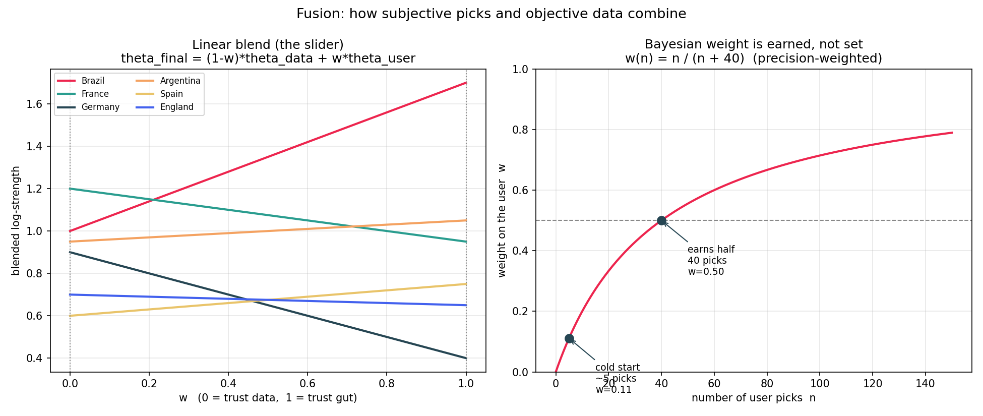
Left: the naïve view, a linear blend with a hand-set slider w. Right: the Bayesian view this project actually uses — w is earned, growing like w(n) = n/(n + const) with the number of picks. Few picks → the data dominates; ~40 well-chosen picks → the user earns roughly half the say. This is the same precision-growth idea behind Glicko's RD and Elo's decaying K.

4.4 Strength → scoreline → bracket

A W/D/L-only model cannot rank a group, because advancement breaks ties on goal difference and goals scored. So fused strengths are turned into goalsvia a Poisson supremacy link (the calibrated baseline rate, home advantage, and scale):

λ_A = e^(μ + home + scale·(θ_A - θ_B))
λ_B = e^(μ - scale·(θ_A - θ_B))

def supremacy_lambdas(theta_a, theta_b, mu, home, scale):
    """Expected goals for each side. `home` is the home-advantage term (0 at a
    neutral venue), added only to the home side's rate."""
    gap = theta_a - theta_b
    lam_a = math.exp(mu + home + scale * gap)
    lam_b = math.exp(mu - scale * gap)
    return lam_a, lam_b

Drawing each side's goals from its Poisson gives the full scoreline distribution — W/D/L and goal difference and goals scored, i.e. every tiebreaker the format needs.

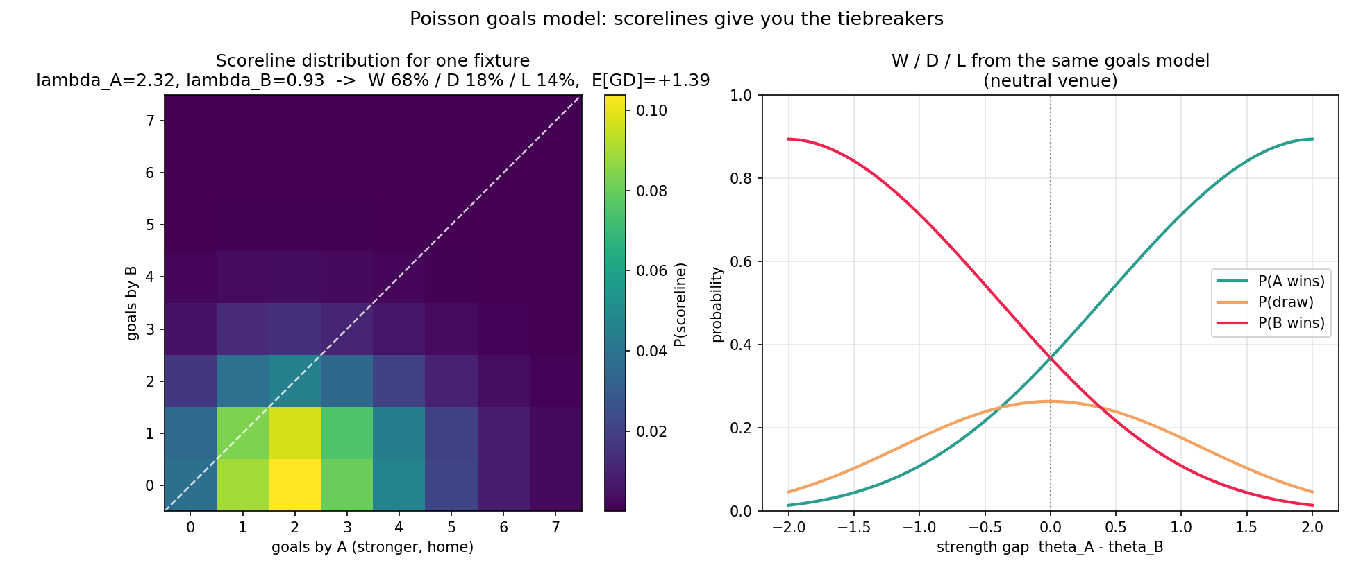
Left: the joint scoreline matrix for one fixture, with win/draw/loss regions. Right: how W/D/L shift as the strength gap changes, all read off the same goals model.

Run that over the group stage and the official knockout structure (Monte Carlo, or an exact bracket DP) and every team gets a per-round reach probability. The differentiator is the contrast:

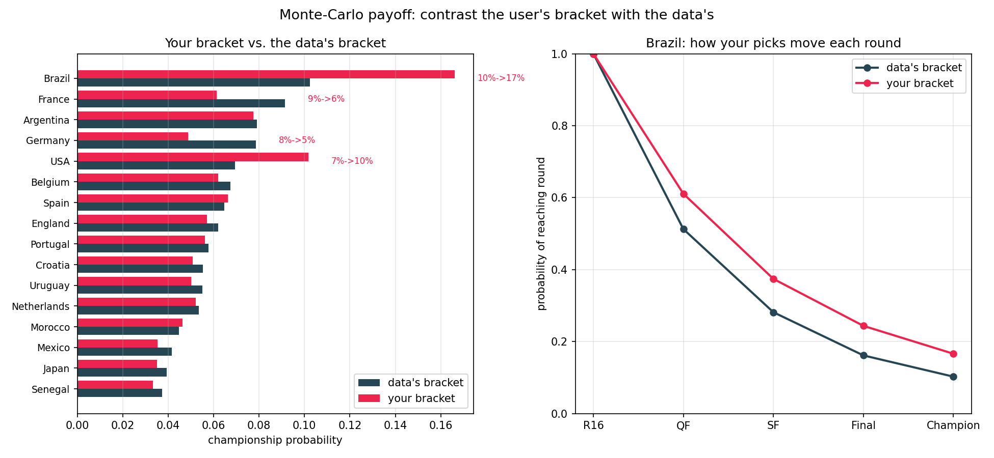
The same bracket simulated with the data strengths vs the user-fused strengths. "The model gives France 14%, your ranking pushes them to 22%" falls straight out of the two runs.

5. How the pairwise comparisons cover enough teams

A 48-team field has C(48,2) = 1128 possible matchups — nobody is clicking through those. The design target is ~40 picks (floor 25, cap 55 — about a normal bracket's effort). The question this section answers: how do so few picks end up covering the field well enough to produce a trustworthy ranking?

Four mechanisms:

5.1 Serve the informative matchups (adaptive pairing)

The Fisher information a single comparison carries about the strength gap is

I = p · (1 - p),   where  p = σ(θ_i - θ_j)

def fisher_information(theta_i, theta_j):
    """Information one comparison carries about the strength gap. Peaks at 0.25
    when p = 0.5 (a coin-flip matchup), ~0 for a blowout."""
    p = sigmoid(theta_i - theta_j)
    return p * (1 - p)

which is maximal at p = 0.5 (a coin-flip matchup, I = 0.25) and ≈ 0 for a blowout. "Brazil vs a minnow" (p ≈ 0.99) teaches almost nothing; a genuine toss-up teaches the most. So the pairing, with probability 1 - ε, serves the most informative not-recently-shown pair (max p(1 - p), i.e. nearest 50/50) given the current fused strengths.

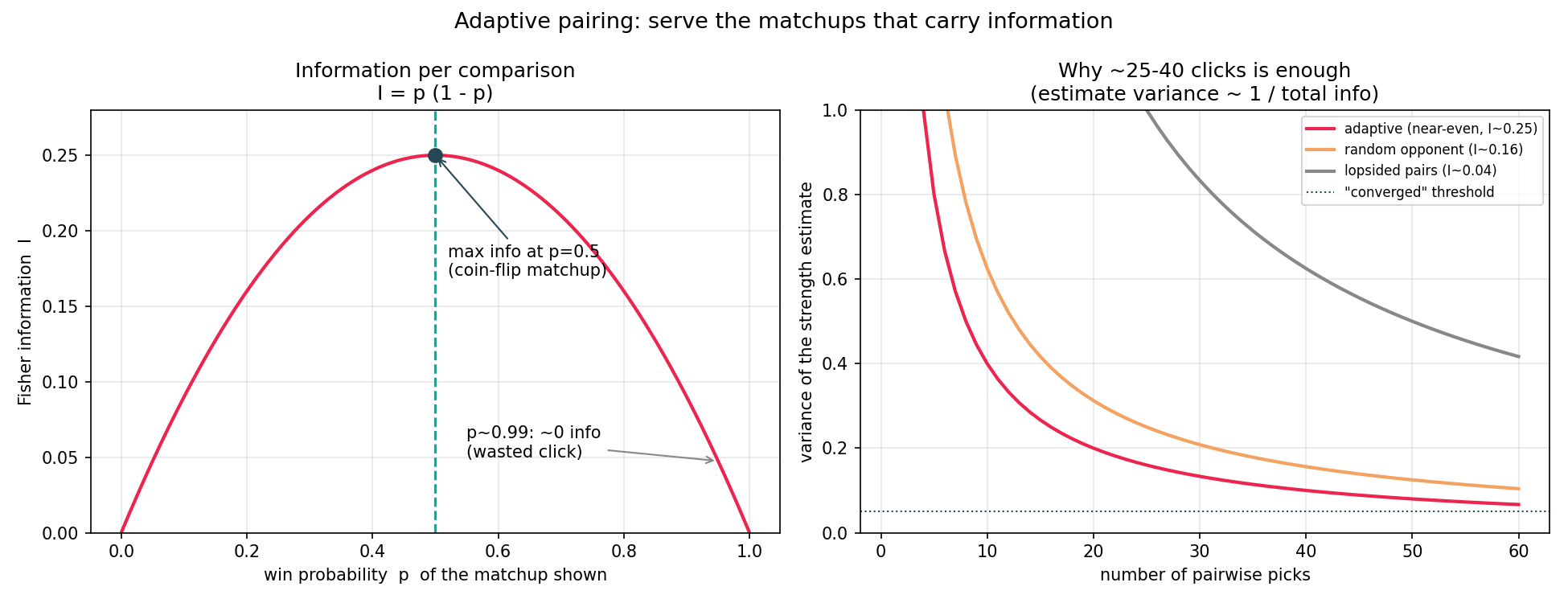
Left: I = p(1 - p) peaks at the coin-flip. Right: because the estimate's variance falls like 1 / (total information collected), always serving near-even pairs (I ≈ 0.25) crosses a "converged" threshold in ~25–40 clicks, where random opponents (I ≈ 0.16) or lopsided ones (I ≈ 0.04) need far more. This is why ~40 picks is enough — they're not 40 random picks, they're 40 maximally informative ones, and they're seeded from the data ratings so the very first matchup is already a real toss-up, not a wasted blowout.

This same p(1 - p) is what becomes τ_user in fusion (§4.3): an informative pick both gets served and earns the user more weight — one quantity, two uses.

5.2 Round-robin the top tier (coverage of the contenders)

Maximizing information alone could orbit a few close pairs and ignore teams the user cares about ranking precisely. So the strongest top 10 teams (by current fused order) are given a large priority bonus for any as-yet-unplayed pair between two of them. Effect: all C(10,2) = 45 top-team matchups get served(most informative first) before the pairing falls back to the wider field. This guarantees the part of the ranking that decides the title — the contenders — is fully covered head-to-head, not sampled.

5.3 Cross-tier anchoring (coverage of the whole field, and dark horses)

With probability ε = 0.18, instead of a near-even pair the engine serves a uniform-random pair — any team, any tier. Two reasons:

• it keeps the user's ranking globally anchored (without it, a chain of

local near-even picks can drift the whole scale); - it lets a dark horse surface and, if the user keeps picking it, climb into the priority tier (§5.2) and get round-robined against the contenders.

The first shown pair is never an anchor — a seeded user should open on a genuinely close matchup, not a random one.

5.4 Information-driven budget (stop when covered, not at a fixed count)

The progress meter is driven by total accumulated Fisher informationΣ_i τ_user[i], not a raw pick count:

• floor 25 — finish unlocks;

• target 40 / progress ≥ 0.92 — "you're locked in";

• cap 55 — hard stop.

Because the meter tracks information, a user who keeps picking near-even contender matchups (high I) fills it fast, while someone clicking obvious blowouts (low I) is nudged toward more useful picks. "Covered enough" is defined by information captured, not clicks spent.

Why it adds up to coverage

• Contenders: fully round-robined (§5.2) → the title-deciding region is

exhaustively compared, not sampled. - Mid/long tail: every team starts pinned to the data prior (§4.3), so an un-compared team isn't "unknown" — it sits at its real strength until the user has reason to move it. - Reach: anchoring (§5.3) periodically pulls in any team, and a team the user champions can climb into the round-robined tier. - Efficiency: each served pick is near-maximally informative (§5.1), so ~40 of them carry the information of hundreds of random comparisons — and the budget stops you the moment that information is in (§5.4).

The net effect: the user explicitly compares the handful of teams whose ranking actually matters, the data prior covers everyone they didn't, and fusion blends the two per team by how much each side earned.